Example of an unbinned maximum likelihood fit with iminuit

Heidelberg University Advanced Lab Course (F-Praktikum)

Ilogo

import numpy as np
import matplotlib.pyplot as plt
from iminuit import Minuit

x = np.loadtxt("https://www.physi.uni-heidelberg.de/Einrichtungen/FP/Datenanalyse/data_ml_fit.txt")

def f(x, a, b):
    """normalized fit function"""
    xmin = -0.95
    xmax = 0.95
    return (6 * (1 + a * x + b * x * x)) / \
            ((xmax - xmin) * (3 * a * (xmax + xmin) + \
            2 * (3 + b * (xmax * xmax + xmax * xmin + xmin * xmin))))

def negative_log_likelihood(a, b):
    p = np.log(f(x, a, b))
    return -np.sum(p)

m = Minuit(negative_log_likelihood, a=1, b=1)
m.errordef = Minuit.LIKELIHOOD

m.migrad()

Migrad
FCN = 606.5		Nfcn = 50
EDM = 2.23e-08 (Goal: 0.0001)
Valid Minimum		No Parameters at limit
Below EDM threshold (goal x 10)		Below call limit
Covariance	Hesse ok	Accurate	Pos. def.	Not forced

	Name	Value	Hesse Error	Minos Error-	Minos Error+	Limit-	Limit+	Fixed
0	a	0.53	0.08
1	b	0.51	0.16

	a	b
a	0.00571	0.00575 (0.476)
b	0.00575 (0.476)	0.0255

# covariance matrix
m.covariance

	a	b
a	0.00571	0.00575 (0.476)
b	0.00575 (0.476)	0.0255

# correlation matrix
m.covariance.correlation()

	a	b
a	1	0.476
b	0.476	1

# function with fitted parameters
xf = np.linspace(-1, 1., 1000)
a_fit = m.values['a']
b_fit = m.values['b']
yf = f(xf, a_fit, b_fit)

plt.hist(x, bins=20, density=True, ec="black", histtype='step');
plt.plot(xf, yf, linewidth=2)
plt.xticks(fontsize=12)
plt.yticks(fontsize=12)
plt.xlabel("x", fontsize=18)
plt.ylabel("f(x; a, b)", fontsize=18);
# plt.savefig("ml_fit_example.pdf")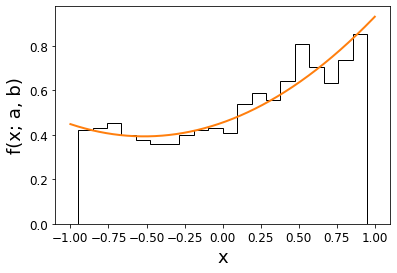

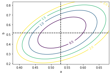
m.draw_contour('a','b');